OBJECTIVE:
We want to test how our media investment performs if we use the budget allocation recommendations. We will compare it against how it would have performed if we had continued allocating the budget as usual.
We will attempt to prove, through statistical analysis, that the budget allocation tool recommendations help to optimize the number of target events with the lowest CPA possible.
To prove this, we will run a 4-week test, using the budget allocation recommendations to allocate media spend. We will compare the performance against a Forecast scenario using historical data.
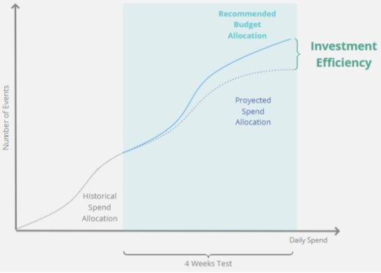
During this test we want to prove the improvement in campaign returns with the Budget Allocation recommendations, in comparison with the projected returns if we had continued allocating the budget as usual.
Methodology:
Forecast Model vs Budget Allocation Model
1) First we use Historical Campaign data as input to build our Forecast Model on the Media investment.
This will help us project how the future number of events and CPA would like for the following 4 weeks if we would have continued to allocate budget as usual.
2) In parallel, we will feed the Budget Allocation Model with the historical data and let it recommend the budget for each media. We will allocate the spend following these recommendations for 4 weeks.
3) We will compare the CPA derived from the Forecast Model allocation vs. the CPA from the BA Model allocation.
It is important that when we get the data from the test client we should corroborate that it is completed and consistent through time and across campaigns/media.
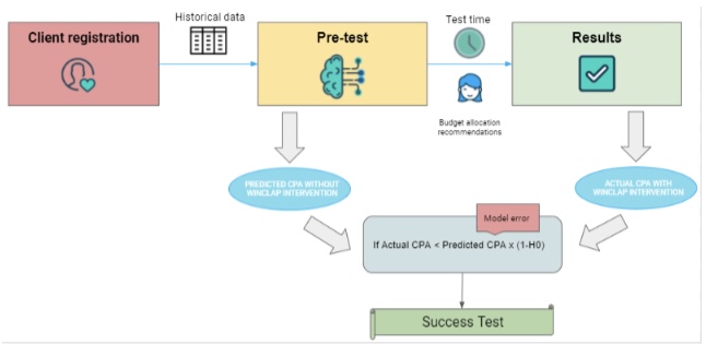
To test our hypothesis we will compare the projected CPA, (obtained after projecting historical data) against the Actual CPA (obtained after following Winclap Budget Allocation recommendations)
BUILDING THE FORECAST MODEL:
We need to incorporate all Paid Media’s historical campaign data into our forecasting model. To Build this model, we will use Facebook’s open-source platform, Prophet.
At this stage, some definitions must be made:
- Define with the client, the target we want to predict. It should be the same target that the BA tool is going to maximize. For example, Paid subscriptions in an App, Ad Revenue, In-app purchases, others.
- Define the regressor.
What are regressors? Regressors are variables that explain the behavior of the variable of interest. (in this case the customer’s Target Event). These variables can be internal such as the volume of certain events from another country or platform or the evolution of marketing spend. Or external variables such as weather, holidays, bitcoin volatility, population mobility behavior, etc.
An example will make this clearer:
Let’s assume we have a shopping app, and our Target Event is the first order a user places after installing the app.
We can infer that our Marketing spends on Paid Media campaigns is a reasonable internal variable to use as a regressor: Increasing our marketing spend attracts more users, which increases the number of first orders.
How to choose the right variables:
Correlation:
To consider the right variables as regressors, we need to make sure there is a correlation between the regressor and the variable of interest.
This means we want to be certain that when the regressor variable changes we observe the variable of interest changing as well.
If we choose as a regressor a variable that has a low correlation with the event variable, we should discard that regressor and consider other variables for this purpose.
Correlation between Spend and Event
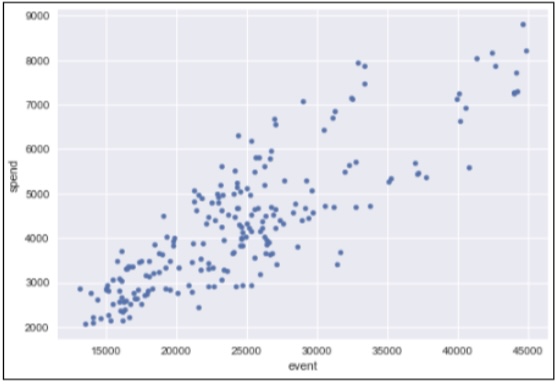
Figure 1: Variables like number of events and spend are usually positively correlated. Increasing the advertising spend tends to increase the number of events (e.g. first orders)
- Spend: The spend is always used as a regressor when analyzing marketing paid campaigns since it is usually the variable that best explains the events/installs of a User Acquisition campaign.
- AppAnnie Data: This data includes competitor information and main metrics in the mobile industry, like downloads, installs, MAUs, etc.
- Trends: we incorporate keywords from Google’s SEM planner (Google Trends and search trends) to find trends that may be correlated with the target variable.
- Miscellaneous Data: Subject to each client’s case, we include specific data sets into the model. For example, Holidays, offline campaigns, weather, bitcoin prices, special events
Once we have defined the regressors and the target variable, it is time to run the model and obtain the predicted values
We broadly divide the analysis of the test into two parts:
- Pre-test: In this instance, the aim is to create a model that predicts the events obtained from the campaigns. Once achieved, the confidence intervals are calculated, giving us as a result the error that we should expect from the model.
- Results:
On one side, our predictions will tell us the events that the client would have achieved if he had continued investing as usual.
On the other side, we will have the actual number of events achieved after allocating the media budget following the model’s recommendation.
In this instance, we seek to validate the alternative hypothesis.
Our Hypothesis: Our Budget Allocation tool improves CPA
Once we have defined our explanatory and target variable, we need to propose the Hypothesis we want to validate.
In this case, our alternative hypothesis (H1) will state that the improvement of the post-test CPA was due to the implementation of the Budget Allocation tool.
The objective of the test is to prove if the alternative Hypothesis stands true or not
For accuracy purposes, we must establish the Confidence intervals.
The Confidence interval expresses how much error we should expect from the predictions. To calculate it, we must indicate the confidence level that the model will perform the predictions optimally. In this case, we will consider that the Budget Allocation tools causally improve CPA if this metric decreases more than XXX% after the test is finished.
H0 = The client’s CPA was not reduced by at least XX% given by the lower confidence limit, with a confidence level of XX%. (see table Z confidence level)
H1 = We reject the null hypothesis, i.e. that the CPA was lowered below the lower confidence limit.
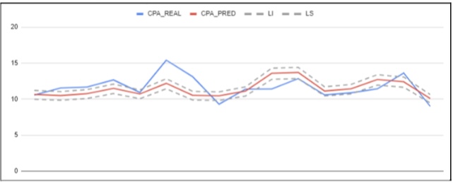
Once we have established the confidence limits, we will plot how the predicted CPA would look compared to the real CPA and, if the latter is within the limits established as the model’s error.
We determine:
- Historical CPA: Spend / Real events
- Predicted CPA: Spend / Forecasted events
Confidence limits for the predicted CPA
FINAL TEST RESULTS
For the duration of the test, the client must allocate its budget following Winclap’s weekly recommendations.
We suggest a test length between 4 to 5 weeks.
It is extremely important for the success of the test that the client performs the allocation as recommended by Winclap, otherwise, it will be difficult to demonstrate the tool’s effectiveness.
Once the pre-test is defined, we run the Budget Allocation tool to get the weekly budget allocation. Our data science manager delivers these recommendations to the client.
We use the Forecast Model projections against the real performance obtained during the test period as contrafactual.
We calculate the difference between the real CPA obtained following the Budget Allocation recommendations and the forecasted CPA as if we would have invested as usual.
We contrast the CPA differences and we check if we have achieved the CPA decrease established in the null hypothesis.
We contrast the following metrics:
- Real CPA: Spend / Real Events (with Winclap Budget Allocation)
- Predicted/Counterfactual CPA: Spend / Forecasted events (with allocation )
We calculate the percentage error between the real CPA and the predicted CPA from these values to evaluate if we can accept our hypothesis.
To accept the hypothesis, the percentage error value must be less than the lower limit proposed. This will conclude that the improvement in the client’s CPA was causal and not casual. In other words, it will prove that the CPA improvement was caused by the Budget Allocation tool and not by other factors.
If we succeed in proving our Hypothesis true, we calculate the final savings for the client and present the results obtained.
CPA: Real vs Predicted
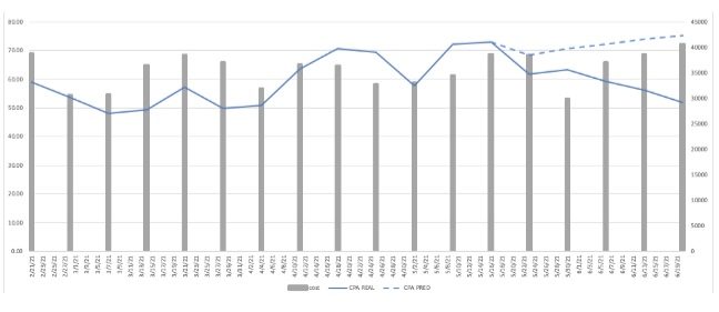
To calculate the final CPA for the client we look at the full test period:
Real CPA= Total Spend / total real events
Predicted CPA= Total Spend/total predicted events
Final check to validate test:
Real CPA<Predicted CPA x (1-H0)
Ready to start using AI to make smarter marketing decisions?

Recent Comments