Introduction

Growth-hacking is a field in marketing focused on growing the most, with the least. It emerged in the context of early-stage startups, who needed massive growth in a short period of time with limited resources. It has since evolved and became part of every marketers playbook across all verticals and company sizes. Paid media occupies a significant portion of the growth effort. When investing in digital advertising, growth hackers aim to get the biggest return from their paid media campaigns. But that is no small task.

In today’s marketing landscape, with advertising inventory proliferating across new media channels, maximizing returns from media spent became a complex, multidimensional problem. Growth marketers not only need to decide the total amount to invest on paid media. Their task has evolved into deciding accurately how to allocate marketing budgets in each combination of country, audience type and ads, across several channels, with the highest returns. But being able to predict the return from each campaign and channel is a challenging task, to say the least. Considering the amount of variables in play, relying solely on marketers’ intuition and experience to get it right, is inefficient and suboptimal.

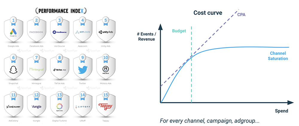
That being said, marketers do not necessarily have to be left only at the mercy of their own intuition to make budget spend decisions. Using the right technology, growth experts can make their media mix decisions easier. AI-based technology can help converting complex campaign analysis into actionable insights, A robust technological solution should be able to integrate multichannel data while simplifying visualization for analysis. It should also find patterns and trends on large historical campaign datasets and provide a recommendation based on these findings.
In search of this promising technology, we’ve tested several external analytics tools to solve this problem. Although some of them provided useful descriptive analytic features, none of them showed clear prescriptive capabilities to suggest an optimal allocation of campaign budgets.

Facing this issue, we realized there was a need to come up with a proprietary solution to optimize budget allocation. With vast experience in Performance Marketing from working with the largest and fastest growing apps from LATAM, and inspired by the teams from Lyft and DoorDash who built similar solutions in-house, we’ve been working for the last year to build a Budget Allocation tool for our Growth Consultancy business. As we realized that our clients could benefit using this platform as well, we have decided to make it available to all marketers.

What is the Budget Allocation Tool about? 

Our tool relies on a Machine Learning infrastructure running algorithms on campaign level datasets to get a  multidimensional optimization between Advertising Spend and Revenue. We aim to predict the amount of revenue (or events) each marketing campaign can drive, based on the amount of spend and other qualitative variables (i.e. country, ad, audience type, among others). We then use these predictions to recommend an optimal budget allocation at the channel and campaign levels. Overall the Budget Allocation process is done in 4 simple steps: 

1. Ingesting historical campaigns data and automatically detecting anomalies.
2. Building a model to define cost curves running predictions for events and revenue, for each campaign on all possible spend levels.
3. Analyzing all possible prediction combinations from Step 2 and selecting the most performant allocation to reach business goals (considering diminishing returns).
4. Re – running the whole process with updated data. 

Over the next sections, we will dive into the process that led us to build the first Budget Allocation model that allows to optimize media mix spend using AI. Allocating budget following the tool’s suggestion, we managed to improve ROAS by 16%. 

Data input

Data Collection and Transformation

In the initial phase, the Data Engineering team at Winclap receives historical performance data from clients’ campaigns. Our infrastructure merges data from multiple sources and summarizes it in simple, user-friendly tables for the Machine Learning models to rely on.

In this example, the data set we are going to use contains tuples of daily spent, installs and revenue derived, for each combination of Ltv.Country, Media.Source, and Audience.Type. The Revenue metric actually refers to Revenue Day 3 to meet with the client criteria. (i.e. revenue cohort 3, the total revenue within the first 3 days after installation).

An exploratory analysis: Getting to know the data 

Once data is structured and summarized, we run a quick exploratory analysis to get a glimpse on how the dataset looks. 

glimpse(in_data) 

## Rows: 379
## Columns: 7
## $ Cohort.Day    <date> 2020-05-14, 2020-05-14, 2020-05-14, 2020-05-14, 2020-0…
## $ Media.Source  <chr> “Facebook Ads”, “Facebook Ads”, “Facebook Ads”, “Facebo…
## $ Ltv.Country   <chr> “AU”, “AU”, “CA”, “CH”, “DK”, “NO”, “SG”, “AU”, “CA”, “…
## $ Audience.Type <chr> “broad”, “lal”, “broad”, “broad”, “broad”, “broad”, “br…
## $ Spend         <dbl> 97.39, 98.09, 80.43, 36.23, 0.53, 30.58, 1.61, 3.28, 42…
## $ Installs      <dbl> 2, 1, 21, 7, 1, 14, 2, 3, 73, 27, 1, 1, 2, 26, 1, 3, 42…
## $ Revenue       <dbl> 0.05, 0.00, 3.06, 0.81, 0.00, 1.15, 0.39, 0.17, 13.49, … 

So far, we count with 379 data points, with 7 columns. One date column Cohort.Day; three categorical: Media.Source, Ltv.Country and Audience.Type, and three numerical: Spend, Installs and the response variable Revenue.

Processing Data and finding correlation between variables: 

With the dataset ready, the Machine Learning algorithms analyze campaigns’ historical data to understand the behavior between multiple variables. 

In this step we will check the spend behavior across different campaigns (Media.Source, Ltv.Country and Audience.Type combination).

ggplot(
in_data,
aes(x = Cohort.Day, y = Spend, color = Ltv.Country, shape = Audience.Type)) +
geom_point() +
geom_line() +
facet_wrap(~Media.Source * Audience.Type) +
theme(axis.text.x = element_text(angle = 45))

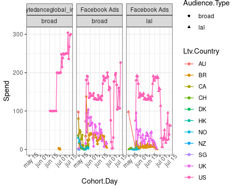
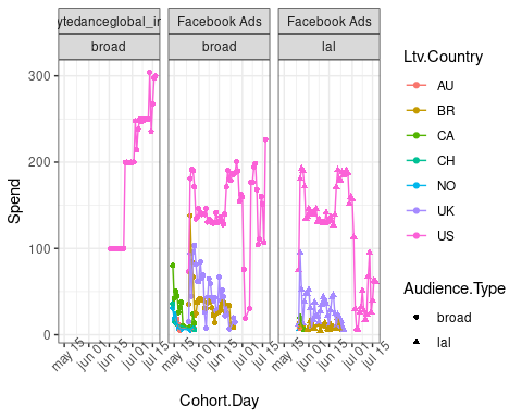
 As we can see in this example, most of the advertisement was placed in the US, a lower amount in the UK and Brazil, and really little money – and for short periods of time- spent on other countries. It should also be noticed that ads on TikTok (bytedanceglobal_int) were only placed for the US, and a few data points for Brazil (SPOILER alert! these few points are going to be further dismissed).

Variables Correlation 

As we want to get the spent allocation which maximizes revenue, it would result interesting to note if there is an individual correlation between any variable and the revenue. 

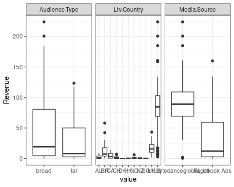
At first glance we can observe a difference in revenue dispersion by country. For the US, UK and Brazil higher revenue variability can be noted, while this is not the case for the rest of the countries . All these findings are not significantly different from what the keen eye of an experienced marketer would get from analyzing the results visually.

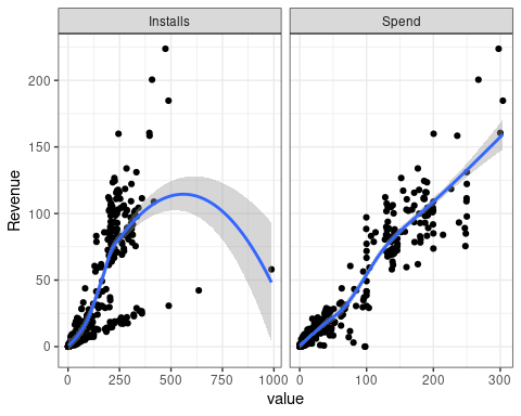
Simple correlation between variables can be observed but this insight is not very useful for decision making. A deeper analysis is needed to understand the extent of this relationship when multiple variables come into play.

It is worth mentioning that for most countries, there are very few samples and with low spend values.  

Observing the correlations between variables, a certain positive correlation is noted between revenue and spend, which is intuitive. It is important to note that even though some variables don’t show correlation by themselves, it is possible that the correlation would appear between interactions of multiple variables.  

In conclusion, the exploratory analysis shows us that:
(i) correlating individual qualitative variables to revenue does not bring incremental insights to decision making, and
(ii) there is an implicit functional relationship between spend and events/revenue, but a deeper analysis is needed to understand the extent of this relationship. 

Based on these initial conclusions, we then run our First Machine Learning models to get a broader comprehension of the relationship between spend and revenue.

Garbage In, Garbage Out

Running the First Machine Learning Model: 

Using an initial set of algorithms, the model attempts to predict how the variable Y (e.g. the Revenue) will behave when the variables X, W, Z (eg. Spend, Country, Media Source, Audience Type) change. 

To assess the model fit, we split the dataset in two: a training set and a validation set. The training set is used to train the different models and select the most accurate one. Finally we contrast our “winning model” versus the validation set and we calculate the error based on the difference between both. At this stage, we are not going to arrive to the optimal solution yet. But rather check how far the model stands from the feasible solution. (in other words, how well it “adjusts” to the validation set). The intuition behind this approach is to get an unbiased evaluation of a final model fit.  

## Model: Revenue ~ Media.Source + Ltv.Country + Audience.Type + Spend 

## Rows of data for test & train – validation – total: 311 – 68 – 379 

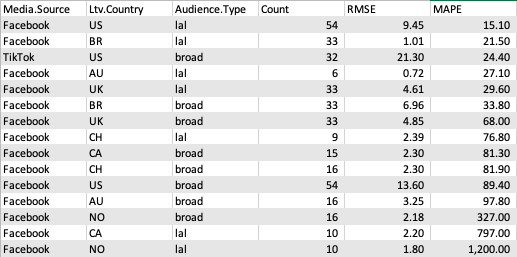
## 47 models trained, best 3:## Validation RMSE – MAPE:  9.49 – 101.06 % 

## Variable importance percentage: 

##   Ltv.Country         Spend  Media.Source Audience.Type
##         51.95         38.10          9.02          0.93 

During this first iteration, we wanted to have a quick observation of the data. We found a Mean Absolute Prediction Error (MAPE) of 101,6%, meaning the model was not adjusting well. This was somehow expected, and made us think about the input data behavior and its reliability. At this point we knew we had some aspects to work on to improve our model to make it fit better. One of those aspects was to identify the presence of outlyers in the dataset which may be adding noise to the relationship between variables.

Outliers Discovery: Understanding the data to adjust the model.  

In Marketing Analytics, we know that outliers may be present all the time. Uncommon extreme observation points in datasets can make it more difficult to understand the relationship between variables at a general level. At this first step we talked to the experts working on the campaigns to acknowledge which data points needed to be excluded from the dataset to avoid “confusing” the model with exceptional data. We asked specifically for those special dates where external efforts and end users behavior could have impacted on the revenue associated with the analyzed campaigns but was not caused by the ad campaign itself. E.g. special Industry events such as Black Friday. 

On next model iterations we will be working on a specific model to detect these outliers and clean the noise from the original dataset. 

Thus, for this analysis we decided to bring some rules to the model to avoid using some data points such as really low spend levels. 

# Remove days with spent lower than $5
sum(in_data$Spend <= 5) 

## [1] 75 

in_data <- filter(in_data, Spend > 5) 

# Calculate outliers detection metrics.
in_data <- in_data %>%
mutate(CPI = Spend / Installs) %>%
mutate(ROI = (Revenue – Spend) / Spend) %>%
mutate(ROAS = Revenue / Spend) %>%
mutate(Profit = Revenue – Spend) %>%
mutate(ARPU = Revenue / Installs) 

ggplot(
pivot_longer(in_data, cols = where(is.numeric)),
aes(name, value)
) +
geom_boxplot() +
facet_wrap(~name, scales = “free”) 

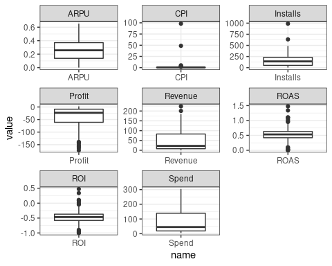
 # 15 * IQR so it is not restrictive.
sum(in_data$CPI > quantile(in_data$CPI, .75) + 15 * IQR(in_data$CPI)) 

## [1] 2 

in_data <- in_data %>%
filter(CPI <= quantile(CPI, .75) + 15 * IQR(CPI)) %>%
select(–CPI, –ROI, –ROAS, –Profit, –ARPU) 

ggplot(
in_data,
aes(x = Cohort.Day, y = Spend, color = Ltv.Country, shape = Audience.Type)
) +
geom_point() +
geom_line() +
facet_wrap(~Media.Source * Audience.Type) +
theme(axis.text.x = element_text(angle = 45)) 

Training the Model and finding the final fit 

Using supervised learning algorithms, the model then adjusts the algorithms to shorten (minimize) the distance between the prediction and the observed value. After multiple iterations, the model finds the algorithm and its hyperparameters that make the best predictions (i.e. the ones with the lowest errors).
Artificial Intelligence becomes relevant here, because the number of calculations and the complexity of them would be too big to grasp using human intelligence alone. (imagine running 1,000 excel functions in one minute) Thus, automatized functions are used to perform these calculations and to adapt as it finds new learning, incorporating them into the algorithms. With each iteration the system adjusts its algorithms ( “learns”) which brings the name Machine Learning.

## Model: Revenue ~ Media.Source + Ltv.Country + Audience.Type + Spend  

## Rows of data for test&train – validation – total: 248 – 54 – 302  

## 36 models trained, best 3:  

##   model     rmse      mae
## 1   GBM 14.70619 9.153505
## 2   GBM 14.77476 8.969904
## 3   GBM 14.95554 9.424402 

## Validation RMSE – MAPE:  13.1 – 21.9 % 

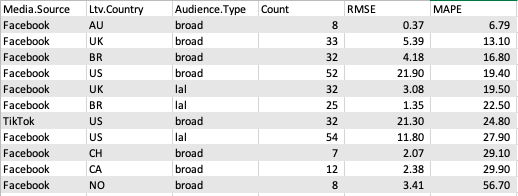
After outliers exclusion and multiple iteration, a fit Model with low MAPE was selected to run predictions.

 ## Variable importance percentage: 

##   Ltv.Country         Spend  Media.Source Audience.Type

##         47.83         40.49         10.57          1.11

On the above chart we have the last model run with a reduced dataset. We deleted outliers and some campaigns that had low volume of data points to analyze. This resulted in a reduction of the MAPE to 21.9% and we decided this was the definite model to run all predictions.

Building cost curves with a working model

At this stage, we already have the model with an acceptable MAPE=21,9% and we need to review the robustness of the predictions before we run the optimal allocations. 

 Here’s a sample plot of how it looks like:

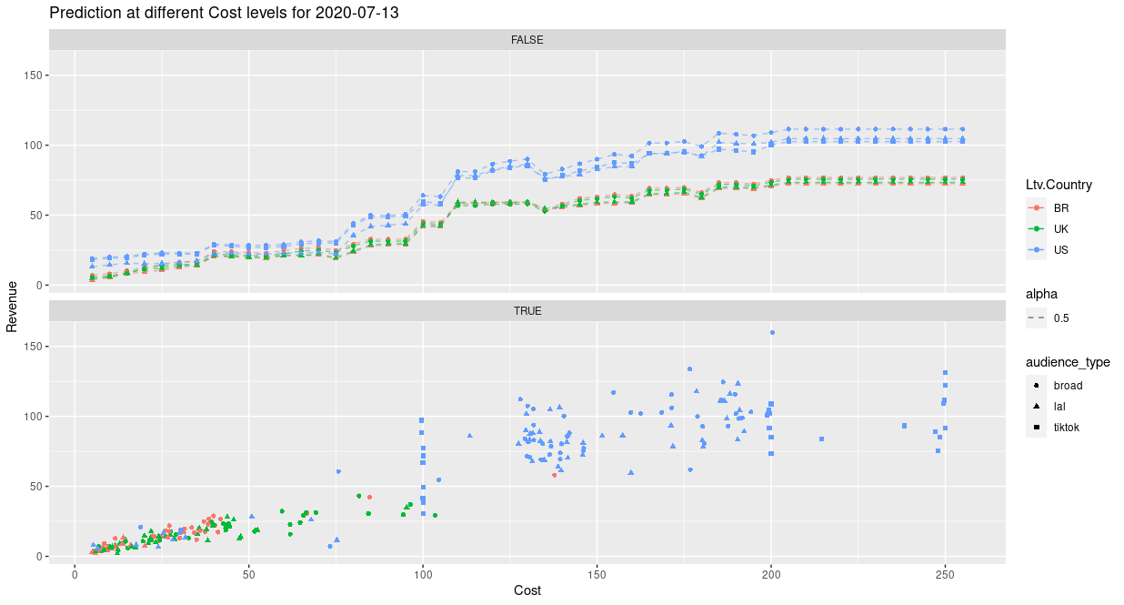
For the different spend levels we want to analyze, we plot all the predictions and get what we call the ‘Cost Curves’. These curves outline the relationship between Cost (spend) and Revenue. Although we get an overall idea of the investment level for all granularities, there is still plenty of information to process to find the optimal budget distribution.

Calculating Optimal Budget Allocation

With cost curves at the campaign level for each channel, our infrastructure is now able to run multiple allocation combinations and find the optimal one. On this stage we run a model to select the best out of 19.487.171 (yes, almost 20M) possible combinations. Once finished, our technology allows us to conclude the analysis with straightforward and clear insights: A simple chart telling you exactly how much you should spend on each campaign to maximize returns.

This chart can be updated automatically. At this first stage we recommend incorporating data to obtain weekly updates on the predictions and allocations. We also recommend to re-train the model every month to account for structural changes in the underlying data.

Conclusions and next steps

Overall It took us 5 weeks to do the analysis, implement the allocations, reach the suggested spend levels and see results to be confident in the model. The results on performance were impressive: 16,9% ROAS improvement and Less than 5% error on prediction.
Currently we are able to run the whole process from data onboarding to budget allocation suggestion in less than 10 days. Our goal is to have the end-to-end process finished in less than 3 days. (data onboarding process is still the most time-demanding step). 

Product Improvement 

We also got significant food for thought for our next iterations on the different components of the product:

 Outliers detection: 

• Can we analyze more data (i.e. organic, benchmarks, additional user behavior from other events) to automate and improve outlier detections?
• Which outliers model (isolation forest, local outliers) can be used and combined to improve the model´s predictive power? 

 Predictions Model: 

• How and which data sets can we incorporate (saturation data, incrementality testing results, seasonality) to improve model accuracy?
• How can we predict spend levels that are farther from historical data?
• How can we test new geos or new channels where there is no historical data?

  Allocations: 

• How can we run more efficient search algorithms to find the optimal allocation and reduce computational effort?
• How can we parallelize the computational effort in the allocations?

Combining years of performance marketing experience with AI led us to a promising start. We will continue working in evolving our models to drive a higher impact on results and help our consultancy growth team as well as marketers around the world to make better budget allocation decisions.

 Isolation Forest: Test different training values and combinations of them; Local outliers: Explore different Parameters such as ‘n_neighbors’